Radar Sensing of Antarctic Ice Sheets
This blog post is by University of Kansas Ph.D. student Shravan Kaundinya.
Radar and Ice
In the field of radioglaciology, a whole host of operating frequencies have been used to study ice. A radar with lower operating frequency (typically less than 1 GHz) ensures greater ability to image the bed and internal layers. By lowering the operating frequency and hence increasing the wavelength of the signal, there is also an increase in required antenna size (thanks to physics!). At frequencies such as 30 and 60 MHz the antenna elements are large, making platform integration challenging. However, at higher frequencies, the antenna size decreases enough to facilitate integration of multiple elements in an array (Figure 1).
In terms of radar system design, an array can be used to electronically scan the antenna beam in postprocessing to view a certain section of the ice more clearly. Each one of the antennas in the array looks at the same area of ice but from a slightly different angle and the signal from each antenna is independently recorded. The latter enables array processing techniques such as swath imaging, which is used for estimating layer slope, 3D imaging the ice bottom, and using layer slope and airborne multipass interferometry to estimate the vertical velocity.
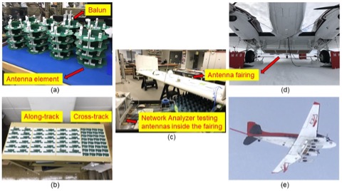
Figure 1: Photos of UHF radar antennas, (a) assembling 64 antenna elements and 128 balun PCB in the lab, (b) soldering 900 components on 128 matching network PCBs, (c) Measuring antennas inside fairing at KU Aerospace Engineering’s Composites Lab, (d) Picture of the antenna fairing on the Basler at Williams Airfield, McMurdo Station, and (e) Picture of the antenna fairing just after take-off at the South Pole
UHF Radar Development
The Center for Remote Sensing and Integrated Systems (CReSIS) at the University of Kansas designed a radar with bandwidth of operation in 600 to 900 MHz and peak transmit power of ~1 kW after losses. The antenna element is a crossed dipole on a square-sized Printed Circuit Board (PCB) and the length of each side is 11.5 cm/4.5 in (Figure 1). Multiple PCBs are placed in a matrix arrangement of 4 rows and 16 columns to form a 64-element antenna array.
The antenna elements are integrated into a fairing that was previously designed and built in-house. The fairing is approximately 3.8 m/12.5 ft in length, 1.3 m/4.3 ft in width, and weighs around 180 kg/400 lb. Four pylons (and eight people!) are used to integrate the fairing to the Basler aircraft.
Each antenna element has two sets of vertical PCBs and one of them is a matching network. It is a circuit with seven components, however for 64 elements and both polarizations, it totals around 900 components (Figure 1). All antenna elements and matching networks were soldered and assembled in-house in three days. For each of the 16 columns, the four elements are combined using a custom power divider. The antennas, power dividers, and all the cabling were finally integrated into the fairing within a week right before shipment day.
The electronics part of the system features a custom designed high-power amplifier stack and novel radar receiver design (Figure 2). The entire system (electronics and antennas) came to fruition through a comprehensive development cycle in less than a year. Designing, machining of enclosures, assembly, integration, and testing of the sub-components and full system was done in-house. The constrained schedule imposed logistical challenges for the equipment, which were successfully navigated thanks to the flexibility of USAP operations.
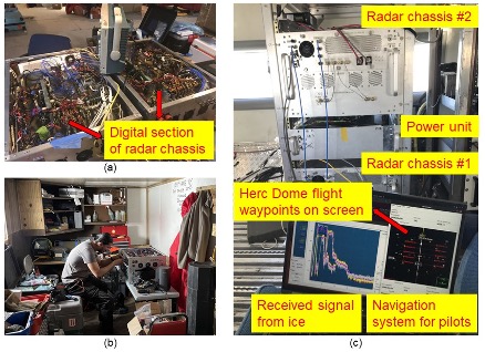
Figure 2: Photos of the UHF radar electronics, (a) Inside the chassis at McMurdo Station, (b) Modifying system at the South Pole, and (c) Radar in operation on the Basler during a science flight
Fieldwork in Antarctica
The electronics chassis was worked on and fine-tuned at McMurdo Station in December 2022. Lab test equipment was used in the field to measure and correct any remaining system issues. However, at the South Pole, survey flights showed inter-system interference between CReSIS’s UHF radar and the University of Texas Institute for Geophysics’ 60 MHz radar. This can be a common occurrence on vessels with numerous scientific instruments. The standard practice includes exercising best-practices during integration followed by extensive testing in the anechoic chamber. However, due to the compressed timeline, we were unable to incorporate all steps and had to do the best with the available options in the field.
Over the course of several days, by making modifications to the system out in the field with limited tools and parts, the interference was gradually reduced. As a result, well-crafted setups were done, like drilling AC-DC power supplies on a wooden plank (obtained from the Great South Pole Dumpster Dive), for convenient power access on the ground and on the aircraft.
Eventually, all major issues were resolved, and multiple missions were flown with all instruments at ~full capability. Preliminary data from the season has been processed and Figure 3 shows a radar echogram from the January 24th, 2023, flight. The figure shows a snapshot of the ice surface, internal layers, and bed along the flow line east of the Dome A region.
For the requirements of the first COLDEX season, the UHF radar has provided sufficient preliminary data for looking at broad areas near Dome A for old ice. Through a tumultuous development year, the team at KU/CReSIS pulled together and executed the plan that made possible what seemed impossible at first (go team! – Figure 4). Modifications and upgrades are currently being performed to get the system ready for test flights in Calgary, Canada in July 2023 and the next field season at the South Pole in December 2023.
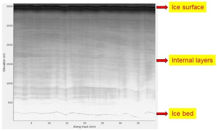
Figure 3: Radar echogram of preliminary data from January 24th, 2023, science flight east of Dome A region near the South Pole
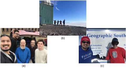
Figure 4: KU/CReSIS team photos in (a) Kansas [L-R, Shravan Kaundinya, Utsa Dey Sarkar, Aaron Paden, Fernando Rodriguez-Morales, and Vincent Occhiogrosso], (b) McMurdo Station [L-R, Lee Taylor, John Paden, Shravan Kaundinya, and Brad Schroeder], and (c) South Pole [L-R, Shravan Kaundinya and John Paden] for COLDEX 2022-2023